The RL community is increasingly pursuing zero logprob mismatch between training and generation, even for day-0 models. This article explains why training/generation parity matters for RL and how Megatron Core and Megatron Inference achieve it within NeMo RL.
Why zero logprob mismatch matters
For policy-gradient methods such as REINFORCE 1, PPO 2, and GRPO 3, logprobs connect the reward of a sampled response to an update of the model parameters. A reward can tell us whether an answer is correct or whether generated code passes its tests, but these checks usually provide no differentiable path back through the sampled tokens.
Let be a prompt, a sampled response, and the model weights. For a reward with no direct dependence on , the policy-gradient identity gives
For a single on-policy response, the basic sampled policy-gradient loss can now be written using token-level estimates with per-token advantagesa:
PPO and GRPO losses
PPO and GRPO use probability ratios to optimize a policy using responses sampled by an earlier policy. Let be the fixed behavior policy that generated the batch.b The token ratio is:
The PPO loss is:
In other words, PPO is trying to maximize the advantage of the sampled tokens, while clipping the advantage to be within a certain range.
For responses sampled from for one prompt, the original response-normalized GRPO loss uses the group advantages defined above and a direct KL penalty: 3
Here . The fixed reference policy , typically the initial SFT model, provides the KL baseline; is the behavior policy that generated the batch. The coefficient controls the penalty. For a given prefix , the KL divergence is
Note that the state usually comes from the inference engine, but plus the loss and gradient computation are done in the training loop. If the training framework (e.g., Megatron Core) cannot produce the same logprob values as the generation engine, there will be numeric incorrectness on the model convergence.
In order to achieve this, there are some techniques to address the numeric issues:
| Technique | Scope | What it establishes |
|---|---|---|
| Determinism | Training | Each repeated runs reproduces itself on the same inputs |
| Batch invariance | Generation | A request's result does not depend on its neighbors |
| Training/generation parity | Both | Both paths produce the same logprobs at the same weights |
In this post, we focus on the third one and discuss how it is implemented in Megatron Core and Megatron Inference with NeMo RL.
NeMo RL recipes
There is a dedicated recipe for zero logprob mismatch in GRPO with Qwen3 in NeMo RL, merged by #3208. It configures Megatron Core, Megatron Inference, and underlying libraries such as Transformer Engine (TE), cuBLAS, and FlashAttention.
Next we're going to why we need these and how they affect the corresponding implementations.
Local arithmetic alignment
First of all, we need to understand the local arithmetic alignment like GEMM, normalization and fused activation.
GEMM and workspace limits
Consider one output element of :
Changing the batch usually changes , while the reduction dimension stays fixed. A different can nevertheless cause the library to choose a different algorithm, including a different partition of the reduction. Floating-point addition does not preserve associativity, so these choices can change the result.
The te_native backend retains native TE/cuBLAS GEMMs and starves their workspace to exclude problematic reduction algorithms, especially split-K variants.
It configures the cuBLAS environment and patches TE's own workspace-size functions, clearing their caches.
These controls reach the model's linear projections, including ordinary MLPs, attention projections, and the LM head. The diagram shows attention/Mamba and dense/MoE paths as architecture alternatives; shared experts are optional.
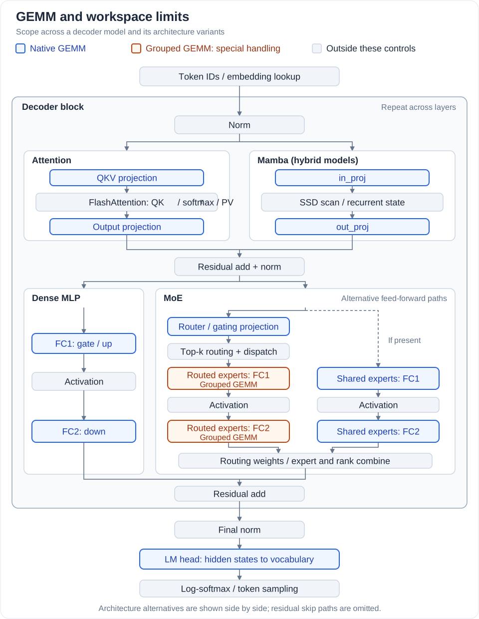
For MoE layers, Megatron Core's optional DeepGEMM path uses BF16 grouped GEMM; te_native keeps native grouped GEMMs.
Each output tile processes the full dimension in a fixed order, while different output tiles can execute independently.
On Hopper, MMA updates FP32 register accumulators.
A full barrier first waits for TMA inputs.
After issuing the MMA instructions for a K block, warpgroup_commit_batch() submits the group and warpgroup_wait<0>() waits for all committed groups to finish before the empty barrier releases the input buffer:
On Blackwell, ordered MMA updates accumulate in FP32 TMEM (Tensor Memory). The third argument below selects the same TMEM accumulator throughout the tile's K loop; the fourth enables accumulation after the first MMA:
The epilogue waits for tmem_full before reading the completed tile; tmem_empty prevents premature reuse of its accumulator storage:
Both paths cast to BF16 after the full reduction and stage the result through shared memory before writing it to global memory.
Attention and token alignment
Training reaches FlashAttention through TE, while generation uses Megatron Inference's dynamic attention path.
Both select FlashAttention 4 and fix num_splits=1.
Split-KV partitions the KV sequence for a query into independently computed segments, then merges their partial outputs using softmax weights.
This adds parallelism when a small decode batch has few queries but long KV sequences.
Setting num_splits=1 disables this partitioning and the cross-segment merge, while still processing K/V in tiles, so that the relative order of K/V tiles for one query should be retained as well.
It removes one source of batch-dependent numerical differences, but can reduce decode performance when split-KV would improve GPU utilization.
Besides, TE RMSNorm can select a different reduction implementation for a different row-count alignment class. Theoratically, RMSNorm should be batch-invariant since the reduction is performed over the last dimension :
Neverthless, the implementation in practice is variant like following:
There are 2 RMSNorm versions in TE 2.18 rmsnorm_fwd_general_kernel and rmsnorm_fwd_tuned_kernel.
The former firstly accumulates and then performs the reduction, while the latter accounts the average and variance first.
Since , they are mathematically equivalent but the float accumulation order is different, leading to different numerical results.
To avoid this, Megatron Core rounds the number of tokens ( dimension) into multiple of 64, and applies this strategy to both eager generation and CUDA-graph token buckets.
The final log-softmax
Even identical logits can produce different logprobs if their normalization uses a different addition tree. Training commonly uses vocab-parallel log-softmax: each TP rank computes local normalization terms, then combines them across ranks. Generation commonly normalizes a complete vocabulary row.
In current NeMo RL implementation, _GenAlignedLogprob / _FullVocabLogprob replace the forward of DistributedLogprob and ChunkedDistributedLogprob:
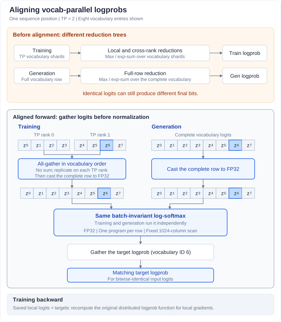
The all-gather concatenates values without summing them. Both sides can then use the same full-row reduction, implemented as one program per row with a fixed 1024-column scanning block. Changing the number of rows does not change how a particular row's columns are grouped.
The cost is additional vocabulary communication, temporary memory, and backward recomputation.
Sequence chunking limits peak memory in the chunked path.
The strict recipe rejects use_fused_linear_logprobs because it bypasses this shared forward.
Megatron Core PR #8421 proposes a separate approach for native vocab-parallel cross entropy: fixed local sums followed by an ordered sum across vocabulary shards.
It does not replace NeMo RL's logprob functions or the engine's log_softmax.
The vocab-parallel cross entropy discussion below explains why these paths still need to be matched explicitly.
Distributed reductions
All-gather, all-to-all, and pipeline send/recv primarily move or reorder values. With a unique source for each element and correct buffer synchronization, packet arrival order does not define a floating-point sum. All-reduce, reduce-scatter, scatter-add, and MoE combine do perform sums, so their grouping, precision, and rounding points need to agree.
TP at a fixed size
Let denote the tensor-parallel size. Current NeMo RL baseline requires the same for training and generation, with a limit of . At TP=2, generation disables the NVLS TP reduction fast path and uses NCCL to match training.
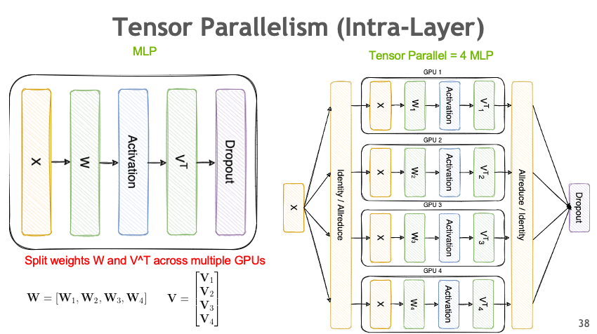
A row-parallel layer produces one partial per rank for each output element. NCCL can change their addition order with message size, chunking, or the element's position in the message. The same token can therefore follow different addition trees in a training batch and a decode batch.
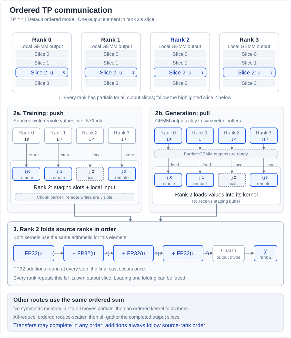
Megatron Core PR #8421 (unmerged; reviewed at 72c11fb) proposes an ordered mode that fixes the order.
For partial from rank , it computes
where is the output dtype. Every FP32 addition still rounds, but the sequence of additions is fixed and there is only one final cast to . The result depends on the partials, rather than where the token sits in the batch.
Training and generation use different data-transfer strategiesc to execute this same sum:
Matching different TP sizes
Fixed rank order alone does not make TP=2 and TP=4 identical. Changing changes each rank's GEMM reduction length from to a different value, so the partials themselves can change before communication begins.
The opt-in batch_invariant_tp_shards=G instead divides the row-parallel reduction dimension into fixed logical shards.
Each shard produces its own GEMM partial , independent of which rank owns it.
For example, with :
| Physical TP size | Shards assigned to each rank |
|---|---|
| Rank 0: ; rank 1: ; rank 2: ; rank 3: | |
| Rank 0: ; rank 1: | |
| Rank 0: |
All three layouts evaluate the same ordered fold, , with the same accumulator precision and final cast. When , each rank computes its partials with one strided batched GEMM. It must retain and communicate the individual partials: pre-summing them within each rank would change the global addition tree. At , the fold is entirely local; at , each rank owns one shard and uses the corresponding single-partial path.
This requires the same on both sides, divisible by each physical TP size, and divisible by . The multi-shard path adds partial-buffer and communication costs, even though the GEMMs remain cuBLAS operations.
Vocab-parallel cross entropy
The PR also makes Megatron Core's native vocab-parallel cross entropy use a fixed reduction for its softmax denominator. For a vocabulary logit , let and let be vocabulary shard . The denominator is computed as
Without an explicit , there is one vocabulary shard per TP rank, so for this calculation.
With batch_invariant_tp_shards=G, the same vocabulary shards are used at every supported TP size.
Both sides must use the same padded vocabulary size, divisible by .
Within each shard, a Triton program uses fixed 1024-lane accumulation followed by a fixed tree sum. Across shards, it uses the ordered fold described above. For ordinary finite logits, the maximum reduction and target-logit selection do not have the same summation-order problem: max is order-independent, and only the target's owning rank contributes a nonzero selected logit.
EP: reproducing the same two-level sum
Expert parallelism (EP) places different experts on different GPUs. For each token, dispatch sends its inputs to the selected experts, and combine adds their contributions back into one output. Compared with the TP reduction above, EP has another level of summation: several selected experts can live on the same rank.
An atomic scatter-add can make the result depend on which contribution arrives first. Even two deterministic implementations can disagree if they use different addition trees. Training and generation must therefore agree on both the local expert sum and the cross-rank sum, including their intermediate casts.
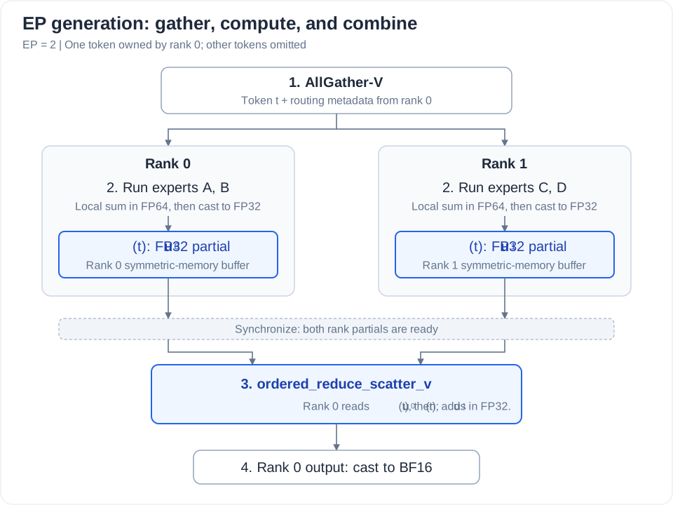
For the common path where routing probabilities have already been applied inside the activation, let be expert 's contribution to token . There is no additional probability multiplication during combine. First, each rank adds its selected experts in fixed expert order using an FP64 accumulator, then casts the partial to FP32. For the ordered set of selected experts on rank :
Second, an FP32 accumulator adds these partials in ascending rank order, then the result is cast to BF16. With EP ranks:
Training dispatches tokens and returns expert outputs through all-to-alld. Its batch-invariant unpermute uses an inverse map from each token to its expert-output rows, so each output reads and adds its own contributions without competing atomic writes. It groups those rows by EP rank and reproduces (2) and (3) inside the combine computation.
Generation with EP greater than 1 uses the NVLS dispatcher:
AllGather-Vcollects variable-count tokens and routing metadata.- Each rank runs its local experts and writes their combined FP32 partials to a symmetric-memory buffer.
- After synchronization makes peer data readable,
ordered_reduce_scatter_vreads the partials and adds source ranks in ascending order using FP32. - Each token's owner receives its combined rows, then casts them to BF16.
Perf tax and results
For Qwen3-30B-A3B at EP=8 and TP=1, Megatron Core PR #6521 and NeMo RL PR #3531 report roughly 1-2% generation overhead with batch invariance and training/generation parity.
These generation measurements do not establish the total GRPO overhead, which depends on the model, parallel layout, and kernel choices.
Validation combines exact token-level logprob comparisons with multi-step synchronous GRPO, requiring gen_kl_error == 0 and token_mult_prob_error == 1 across weight updates.
NeMo RL PR #4683 reports about 248,000 response tokens with identical training/generation logprobs over five steps for a Nemotron Nano v3 30B-A3B MXFP8 configuration with sequence packing.
Footnotes
-
Ronald J. Williams (1992), Simple statistical gradient-following algorithms for connectionist reinforcement learning, Machine Learning 8, 229-256. ↩
-
John Schulman et al. (2017), Proximal Policy Optimization Algorithms, arXiv:1707.06347. ↩
-
Zhihong Shao et al. (2024), DeepSeekMath: Pushing the Limits of Mathematical Reasoning in Open Language Models, arXiv:2402.03300; introduces Group Relative Policy Optimization. ↩ ↩2